Distributed Control & Second-Order Consensus for UAV Swarms

Introduction#

This article presents a distributed control framework for multi-UAV formation systems, built on the ROS2+PX4 simulation environment and Multi-Drone Offboard Control foundations. By integrating ROS2’s distributed communication architecture with PX4’s MAVLink protocol, the system enables real-time state sharing and cooperative control across multiple drones. The consensus-based control law allows each drone to rely solely on local neighbor information to achieve formation keeping and trajectory tracking, offering a highly reliable inter-drone communication method for large-scale swarm missions.

UAV formation control generally falls into two architectural paradigms: centralized and distributed. Their differences lie primarily in decision hierarchy, communication topology, and system robustness.

Centralized control relies on a single central node (e.g., a ground station or a lead UAV) for global decision-making. All drones execute commands issued by this central node. It offers high control precision and excellent formation consistency, making it suitable for complex missions. However, it suffers from single-point failure risk, high communication load on the central node, and poor scalability — especially critical when the central node fails or comes under attack, which can severely compromise formation safety.

Distributed control has no central node. Each drone makes autonomous decisions through local communication, interacting only with neighboring drones. This approach provides strong robustness, high scalability, and dynamic adaptability for large-scale formations, at the cost of higher coordination complexity and weaker global optimization capability.

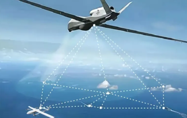
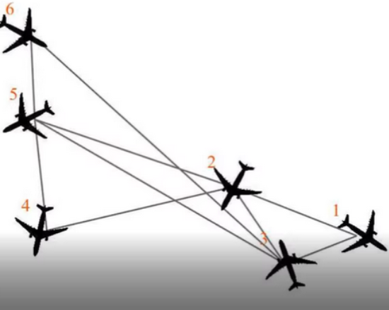
Centralized communication diagram — Figure 1: Centralized communication -- single node broadcasts messages

Distributed communication diagram — Figure 2: Distributed communication -- multiple nodes exchange messages pairwise

This article is based on a formation of six UAVs. We first establish a first-order swarm cooperative control law, then extend it to a more general second-order model (acceleration input), solve for the feedback gain matrix via the LMI method, and finally validate the approach in Gazebo simulation. The final section provides a rigorous proof of the error dynamics under constant formation offsets.

Mathematical Preliminaries#

Extensive literature exists on the mathematical background of distributed cooperative control systems; this section only provides the necessary review. Readers are referred to the following for deeper understanding:

Graph theory fundamentals: Multi-Agent System Control (1) — Graph Theory ↗ (Chinese)
Properties of the Laplacian matrix: CSDN Blog ↗ (Chinese)
Consensus control lemmas: CSDN Blog ↗ (Chinese), which can be used to prove the convergence of the control law

From a theoretical perspective, it can be shown that the swarm cooperative system constructed in this article is capable of achieving cooperative UAV formation tasks.

First-Order Consensus Control#

System Model#

Consider a formation of $N+1$ UAVs. The drone labeled $0$ is the leader, and the remaining $N$ drones labeled $i = 1, 2, \dots, N$ are followers.

Each drone uses a first-order kinematic model in which the state consists only of position information. Let $p_i \in \mathbb{R}^3$ denote the position of drone $i$ , and let the control input be a velocity command $v_i \in \mathbb{R}^3$ :

\dot{p}_i = v_i

First-Order Consensus Protocol#

We adopt the classical linear consensus protocol, where the control input of drone $i$ is determined by the weighted sum of neighbor state deviations:

v_i = k_p \sum_{j \in \mathcal{N}_i} w_{ij}(p_j - p_i)

where $\mathcal{N}_i$ is the neighbor set of drone $i$ , $w_{ij} \ge 0$ are communication weights, and $k_p > 0$ is the position gain.

For a connected graph, it can be proved that the position states satisfy $p_i(t) - p_j(t) \to 0$ as $t \to \infty$ , meaning all followers asymptotically converge to the leader’s position. This is the most fundamental application of distributed consensus in swarm formation — global position synchronization achieved using only local neighbor position deviations.

Second-Order Distributed Control#

Theoretical Modeling#

Single-UAV Dynamics#

We consider a formation of $N+1$ UAVs. Drone $0$ serves as the leader, chosen as a virtual leader (not physically flying). Drones labeled $i = 1, 2, \dots, N$ are followers.

Each drone is modeled with second-order dynamics (containing both position and velocity states). The state of drone $i$ is:

\xi_i = \begin{bmatrix} p_i \\ v_i \end{bmatrix} \in \mathbb{R}^6, \quad p_i \in \mathbb{R}^3, \quad v_i \in \mathbb{R}^3

where $p_i$ is the position and $v_i$ is the velocity. The control input is a second-order acceleration command $u_i \in \mathbb{R}^3$ .

The linearized second-order model of each drone can be written in matrix form:

\dot{\xi}_i = A \xi_i + B u_i \tag{1}

The matrices $A \in \mathbb{R}^{6 \times 6}$ and $B \in \mathbb{R}^{6 \times 3}$ are block matrices, obtained by simple derivation:

\dot{\xi}_i = \begin{bmatrix} \dot{p}_i \\ \dot{v}_i \end{bmatrix} = \begin{bmatrix} v_i \\ u_i \end{bmatrix} = \begin{bmatrix} 0_{3\times3} & I_3 \\ 0_{3\times3} & 0_{3\times3} \end{bmatrix} \begin{bmatrix} p_i \\ v_i \end{bmatrix} + \begin{bmatrix} 0_{3\times3} \\ I_3 \end{bmatrix} u_i

\Rightarrow A = \begin{bmatrix} 0_{3\times3} & I_3 \\ 0_{3\times3} & 0_{3\times3} \end{bmatrix}, \quad B = \begin{bmatrix} 0_{3\times3} \\ I_3 \end{bmatrix} \tag{2}

Linear Consensus Protocol#

We adopt the classical linear consensus protocol, where the input of each follower drone ( $i = 1, 2, \dots, N$ ) can be expressed as the weighted sum of neighbor state deviations:

u_i = K \sum_{j=0}^{N} w_{ij}(\xi_j - \xi_i) \tag{3}

where $K$ is the state-feedback gain matrix.

Rewrite this in Laplacian matrix form. Define the weight matrix $W = (w_{ij})$ , degree matrix $D = \text{diag}(d_0, \dots, d_N)$ where $d_i = \sum_j w_{ij}$ , and Laplacian matrix $L = D - W$ whose entries satisfy $l_{ii} = \sum_{j=0}^N w_{ij}$ , $l_{ij} = -w_{ij}$ ( $i \ne j$ ), $w_{ii} = 0$ .

Expand equation (3):

\begin{aligned} u_i &= K \sum_{j=0}^{N} w_{ij}(\xi_j - \xi_i) \\ &= K\left( \sum_{j=0}^{N} w_{ij} \xi_j - \left(\sum_{j=0}^{N} w_{ij}\right)\xi_i \right) \\ &= K\left( \sum_{j=0, j \ne i}^{N} w_{ij} \xi_j + w_{ii}\xi_i - \left(\sum_{j=0}^{N} w_{ij}\right)\xi_i \right) \\ &= K\left( -\sum_{j=0, j \ne i}^{N} l_{ij} \xi_j + 0 - l_{ii}\xi_i \right) \\ &= -K \sum_{j=0}^{N} l_{ij} \xi_j \end{aligned}

Therefore:

u_i = -K \sum_{j=0}^{N} l_{ij} \xi_j, \quad i = 1, 2, \dots, N \tag{4}

Error System Definition#

Define the error of each follower relative to the leader (labeled $0$ ):

e_i = \xi_i - \xi_0, \quad i = 1, \dots, N \tag{5}

From the single-drone dynamics (equation (1)):

\dot{e}_i = \dot{\xi}_i - \dot{\xi}_0 = A\xi_i + Bu_i - \dot{\xi}_0

Substitute the control law (equation (4)):

\dot{e}_i = A\xi_i - BK\sum_{j=0}^{N} l_{ij} \xi_j - \dot{\xi}_0

For all $j \ge 1$ , we have $\xi_j = e_j + \xi_0$ . Split into $j=0$ and $j \ge 1$ :

\sum_{j=0}^{N} l_{ij} \xi_j = \sum_{j=1}^{N} l_{ij} e_j + \left(l_{i0} + \sum_{j=1}^{N} l_{ij}\right)\xi_0

Using the Laplacian’s zero row-sum property $\sum_{j=0}^N l_{ij} = 0$ , we therefore have $l_{i0} + \sum_{j=1}^N l_{ij} = 0$ , so:

\sum_{j=0}^{N} l_{ij} \xi_j = \sum_{j=1}^{N} l_{ij} e_j

Substituting back yields the error dynamics for a single follower $i$ :

\dot{e}_i = A e_i - BK \sum_{j=1}^{N} l_{ij} e_j + (A\xi_0 - \dot{\xi}_0) \tag{6}

Stack all $N$ followers:

e = \begin{bmatrix} e_1 \\ \vdots \\ e_N \end{bmatrix} \in \mathbb{R}^{6N}, \quad d = \mathbf{1}_N \otimes \left(A\xi_0 - \dot{\xi}_0\right) \in \mathbb{R}^{6N}, \quad \tilde{L} = [-l_{ij}]_{i,j=1}^N

Writing the error dynamics in matrix form:

\dot{e} = \left(I_N \otimes A + \tilde{L} \otimes BK\right) e + d \tag{7}

Lyapunov Function and LMI Condition#

Choose the Lyapunov function $V(e) = e^\top P e$ , where $P = I_N \otimes X^{-1}$ and $X \succ 0$ is a symmetric positive-definite matrix:

V(e) = e^\top \left(I_N \otimes X^{-1}\right) e \tag{8}

The closed-loop system (homogeneous part) of the error dynamics is:

\dot{e} = A_{cl} e, \quad A_{cl} = I_N \otimes A + \tilde{L} \otimes BK \tag{9}

Compute the Lyapunov derivative:

\dot{V} = e^\top \left( A_{cl}^\top P + P A_{cl} \right) e

To guarantee asymptotic stability, we require $\dot{V} \prec 0$ , i.e.:

A_{cl}^\top P + P A_{cl} \prec 0 \tag{10}

Congruence Transformation Note: Let $S \in \mathbb{R}^{n \times n}$ be a symmetric matrix and $M \in \mathbb{R}^{n \times n}$ be an invertible matrix. Define $\bar{S} = M S M^\top$ . Then $S \succ 0 \iff \bar{S} \succ 0$ and $S \prec 0 \iff \bar{S} \prec 0$ . For any nonzero vector $z$ , $z^\top \bar{S} z = (M^\top z)^\top S (M^\top z)$ , and since $M$ is invertible the sign is preserved.

Apply the congruence transformation to eliminate $X^{-1}$ :

\bar{S} = (I_N \otimes X) \left( P A_{cl} + A_{cl}^\top P \right) (I_N \otimes X)

Then $P A_{cl} + A_{cl}^\top P \prec 0 \iff \bar{S} \prec 0$ . Expanding $\bar{S}$ :

\bar{S} = I_N \otimes (AX + XA^\top) + \tilde{L} \otimes (BKX) + \tilde{L}^\top \otimes \big(X(BK)^\top\big) \tag{11}

Apply the variable substitution $Y = KX$ to eliminate bilinear coupling:

BKX = BY, \quad X(BK)^\top = (BY)^\top

Thus the LMI condition is:

I_N \otimes (AX + XA^\top) + \tilde{L} \otimes (BY) + \tilde{L}^\top \otimes (BY)^\top \prec 0, \quad X \succ 0 \tag{12}

Control Law with Formation Offsets#

Assume the formation has desired relative positions. Define $r_{ij}$ as the desired relative offset between follower $i$ and follower $j$ . The control law is modified to:

u_i = K \sum_{j=0}^{N} w_{ij} \big[(\xi_j - \xi_i) + r_{ij}\big] = -K \sum_{j=0}^{N} l_{ij} \xi_j + K \sum_{j=0}^{N} w_{ij} r_{ij} \tag{13}

Redefine the error term. Let $r_{ij} = r_i - r_j$ (with $r_0 = 0$ ), where $r_i$ is the desired formation position offset of follower $i$ relative to the leader. Define the new error as:

e_i = \xi_i - (\xi_0 + r_i), \quad i = 1, \dots, N

Differentiate the error, substituting the single-drone dynamics (1) and the control law (13):

\dot{e}_i = A\xi_i - BK \sum_{j=0}^{N} l_{ij} \xi_j + BK \sum_{j=0}^{N} w_{ij} r_{ij} - \dot{\xi}_0 - \dot{r}_i \tag{14}

Simplify Sum 1 (Laplacian term). For $j \ge 1$ , substitute $\xi_j = e_j + \xi_0 + r_j$ , and $\xi_0 = \xi_0 + r_0$ :

\begin{aligned} \sum_{j=0}^{N} l_{ij} \xi_j &= l_{i0} \xi_0 + \sum_{j=1}^{N} l_{ij} (e_j + \xi_0 + r_j) \\ &= \sum_{j=1}^{N} l_{ij} e_j + \Big(l_{i0} + \sum_{j=1}^{N} l_{ij}\Big) \xi_0 + \sum_{j=1}^{N} l_{ij} r_j \end{aligned}

From the Laplacian zero row-sum property ( $\sum_{j=0}^N l_{ij} = 0$ ), we obtain $l_{i0} + \sum_{j=1}^N l_{ij} = 0$ , hence:

\sum_{j=0}^{N} l_{ij} \xi_j = \sum_{j=1}^{N} l_{ij} e_j + \sum_{j=1}^{N} l_{ij} r_j \tag{15}

Simplify Sum 2 (formation weighting term). Using $r_{ij} = r_i - r_j$ , $w_{ii} = 0$ , and $l_{ij} = -w_{ij}$ ( $i \ne j$ ):

\begin{aligned} \sum_{j=0}^{N} w_{ij} r_{ij} &= \sum_{j=0}^{N} w_{ij}(r_i - r_j) = r_i \sum_{j=0}^{N} w_{ij} - \sum_{j=0}^{N} w_{ij} r_j \\ &= l_{ii} r_i - \sum_{j=0, j \ne i}^{N} w_{ij} r_j = l_{ii} r_i + \sum_{j=0, j \ne i}^{N} l_{ij} r_j = \sum_{j=0}^{N} l_{ij} r_j \end{aligned}

Therefore:

\sum_{j=0}^{N} w_{ij} r_{ij} = \sum_{j=0}^{N} l_{ij} r_j \tag{16}

Substitute into the error equation. Substitute $\xi_i = e_i + \xi_0 + r_i$ (for $i \ge 1$ ), along with (15) and (16), into (14). After expansion, note that the $BK \sum_{j=1}^N l_{ij} r_j$ term and the $BK \sum l_{ij} r_j$ term (the part with $j \ge 1$ ) cancel each other, and $r_0 = 0$ means $BK l_{i0} r_0 = 0$ . The result is:

\dot{e}_i = A e_i - BK \sum_{j=1}^{N} l_{ij} e_j + (A\xi_0 - \dot{\xi}_0) + (A r_i - \dot{r}_i) \tag{17}

Constant offset case — LMI condition unchanged. If $r_i$ is a constant position offset (the most common case), i.e.:

r_i = \begin{bmatrix} p_{r_i} \\ 0 \end{bmatrix}, \quad \dot{r}_i = 0, \quad A = \begin{bmatrix} 0 & I \\ 0 & 0 \end{bmatrix} \Rightarrow A r_i = \begin{bmatrix} 0 \\ 0 \end{bmatrix}

The extra bias term $(A r_i - \dot{r}_i)$ vanishes, and the error dynamics reduce to the classic homogeneous form:

\dot{e}_i = A e_i - BK \sum_{j=1}^{N} l_{ij} e_j + (A\xi_0 - \dot{\xi}_0) \tag{18}

Stacking all followers:

\dot{e} = \left(I_N \otimes A + \tilde{L} \otimes BK\right) e + \mathbf{1}_N \otimes (A\xi_0 - \dot{\xi}_0) \tag{19}

This is identical to equation (7). Therefore, when formation-internal relative positions (constant offsets) are present, the Lyapunov analysis and LMI condition (12) remain unchanged.

Simulation Implementation#

Solving the LMI Inequality#

The above LMI condition is solved in MATLAB using the YALMIP toolbox. The chosen communication topology is: drone $0$ is the virtual leader, drone $1$ subscribes to drones $0$ , $2$ , and $3$ (relative formation position $(0, 0)$ ), drone $2$ subscribes to drone $1$ (relative formation position $(-5, -10)$ ), and drone $3$ subscribes to drone $1$ (relative formation position $(5, -10)$ ).

% ------------ Parameters ------------
N = 3;               % Number of followers
% System matrices A (6x6) and B (6x3)
A = [zeros(3) eye(3); zeros(3) zeros(3)];
B = [zeros(3); eye(3)];

% Construct L_sub and Ltilde
L_sub = [ 3 -1 -1;
         -1  1  0;
         -1  0  1 ];
Ltilde = -L_sub;

% ------------- YALMIP Variables -------------
n = size(A,1);      % =6
m = size(B,2);      % =3

X = sdpvar(n,n,'symmetric');    % X ≻ 0
Y = sdpvar(m,n,'full');         % Y = K*X (m x n)

% Construct large matrix S = I_N ⊗ (A X + X A') + Ltilde ⊗ (B Y) + Ltilde' ⊗ (B Y)'
S = kron(eye(N), A*X + X*A') + kron(Ltilde, B*Y) + kron(Ltilde', (B*Y)');

% LMI: S < 0, X > 0
eps = 1e-6;
Constraints = [S <= -eps*eye(N*n), X >= eps*eye(n)];
Constraints = [Constraints, X == X'];

% ------------- Solve -------------
options = sdpsettings('verbose', 1, 'solver', 'sedumi');
Objective = [];
sol = optimize(Constraints, Objective, options);

if sol.problem == 0
    Xopt = value(X);
    Yopt = value(Y);
    K = Yopt * (Xopt \ eye(n));   % K = Y * X^{-1}
    disp('Found feasible K:');
    disp(K);
else
    disp('Solver failed; return information:');
    yalmiperror(sol.problem)
end

matlab

The solution for the formation positions used in this article (readers should solve according to their own models):

Found feasible K:
    0.6983    0.0000    0.0000    2.1929    0.0000    0.0000
   -0.0000    0.6983    0.0000   -0.0000    2.1929    0.0000
    0.0000   -0.0000    0.6983   -0.0000   -0.0000    2.1929

plaintext

Hence $K_p = 0.6983$ , $K_v = 2.1929$ .

From Acceleration to Velocity Commands#

PX4 employs a typical cascaded PID control structure: position controller → velocity controller → acceleration controller → attitude controller → angular rate controller → motors.

If one were to directly use second-order acceleration input, gravity compensation and attitude resolution would be required to convert world-frame acceleration commands into body-frame attitude commands:

a_{body}^{des} = R_b^{w^{-1}} \left( a_{world}^{des} - g \right)

In Offboard mode, direct acceleration control is uncommon in engineering practice (for instance, $a_z = 0$ does not produce hover; a gravity compensation empirical value must be provided).

Therefore, in this article the virtual acceleration command obtained from the linear consensus protocol is integrated to generate the desired velocity input:

a_i(k) = k_p \sum_{j \in \mathcal{N}_i} \big(p_j(k) - p_i(k) + r_{ij}(k)\big) + k_v \sum_{j \in \mathcal{N}_i} \big(v_j(k) - v_i(k)\big) \tag{20}

v_i^{des}(k+1) = v_i^{des}(k) + a_i(k) \Delta t \tag{21}

The result is then smoothed through a first-order filter:

v_i^{cmd}(k+1) = \alpha v_i^{des}(k+1) + (1 - \alpha) v_i^{cmd}(k) \tag{22}

where $\alpha \in (0, 1)$ is the filter factor, set to $0.5$ in this article.

Code example for the $x$ and $y$ directions:

float ax = position_gain_ * sum_dx + velocity_gain_ * sum_dvx;
float ay = position_gain_ * sum_dy + velocity_gain_ * sum_dvy;

float vx_integrated = desired_velocity_[0] + ax * dt;
float vy_integrated = desired_velocity_[1] + ay * dt;

desired_velocity_[0] = filter_alpha_ * vx_integrated
                     + (1.0f - filter_alpha_) * desired_velocity_[0];
desired_velocity_[1] = filter_alpha_ * vy_integrated
                     + (1.0f - filter_alpha_) * desired_velocity_[1];

cpp

This approach preserves the dynamic characteristics of second-order consensus control while being compatible with PX4’s velocity control layer, offering good engineering feasibility and stability.

Filter Discretization Derivation#

The continuous-time first-order low-pass filter equation is:

\tau \dot{v}_f(t) + v_f(t) = v(t)

where $v_f(t)$ is the filtered velocity signal, $v(t)$ is the input signal, and $\tau$ is the time constant. Rewriting:

\dot{v}_f(t) = \frac{1}{\tau}\big(v(t) - v_f(t)\big)

Under discrete conditions with sampling period $dt$ :

\dot{v}_f(t) \approx \frac{v_f[k] - v_f[k-1]}{dt}

Substituting:

\frac{v_f[k] - v_f[k-1]}{dt} = \frac{1}{\tau}\big(v[k] - v_f[k-1]\big)

Multiplying both sides by $dt$ and rearranging:

v_f[k] - v_f[k-1] = \frac{dt}{\tau}\big(v[k] - v_f[k-1]\big)

Define $\alpha = \frac{dt}{\tau + dt}$ , yielding:

v_f[k] = (1 - \alpha) v_f[k-1] + \alpha v[k] \tag{23}

This matches the form of equation (22).

ROS2 Coordinate Transformation Note#

In a ROS2 + PX4 launch, each drone instance by default starts with its own takeoff point as the origin $(0, 0)$ . Therefore, each time a position is received in a subscription callback, one must manually subtract the takeoff point coordinates to obtain the global coordinates before substituting into the control law. A code example is provided in the next section.

Reference Code#

The following is the complete C++ code for UAV $1$ (which subscribes to the virtual leader as well as neighboring UAVs $2$ and $3$ ), corresponding to the model described above. The code for UAVs $2$ and $3$ is similar, requiring only modifications to the subscription topology and formation offsets.

#include <rclcpp/rclcpp.hpp>
#include <px4_msgs/msg/offboard_control_mode.hpp>
#include <px4_msgs/msg/trajectory_setpoint.hpp>
#include <px4_msgs/msg/vehicle_command.hpp>
#include <px4_msgs/msg/vehicle_odometry.hpp>
#include <vector>
#include <map>
#include <array>
#include <limits>
#include <chrono>

struct NeighborState {
    std::array<float, 3> position = {0.0f, 0.0f, 0.0f};
    std::array<float, 3> velocity = {0.0f, 0.0f, 0.0f};
    bool valid = false;
};

class UAV1Controller : public rclcpp::Node {
public:
    UAV1Controller() : Node("uav1_controller") {
        rclcpp::QoS qos(10);
        qos.reliability(RMW_QOS_POLICY_RELIABILITY_BEST_EFFORT);
        qos.durability(RMW_QOS_POLICY_DURABILITY_TRANSIENT_LOCAL);
        qos.history(RMW_QOS_POLICY_HISTORY_KEEP_LAST);

        offboard_control_mode_publisher_ = create_publisher<
            px4_msgs::msg::OffboardControlMode>(
            "/px4_1/fmu/in/offboard_control_mode", qos);
        trajectory_setpoint_publisher_ = create_publisher<
            px4_msgs::msg::TrajectorySetpoint>(
            "/px4_1/fmu/in/trajectory_setpoint", qos);
        vehicle_command_publisher_ = create_publisher<
            px4_msgs::msg::VehicleCommand>(
            "/px4_1/fmu/in/vehicle_command", qos);

        own_odometry_sub_ = create_subscription<
            px4_msgs::msg::VehicleOdometry>(
            "/px4_1/fmu/out/vehicle_odometry", qos,
            [this](const px4_msgs::msg::VehicleOdometry::SharedPtr msg) {
                own_position_ = {msg->position[0], msg->position[1],
                                 msg->position[2]};
                own_velocity_ = {msg->velocity[0], msg->velocity[1],
                                 msg->velocity[2]};
                own_state_valid_ = true;
            });

        uav2_sub_ = create_subscription<px4_msgs::msg::VehicleOdometry>(
            "/px4_2/fmu/out/vehicle_odometry", qos,
            [this](const px4_msgs::msg::VehicleOdometry::SharedPtr msg) {
                neighbor_states_[2] = {
                    {msg->position[0] - 5.0f, msg->position[1] - 10.0f,
                     msg->position[2]},
                    {msg->velocity[0], msg->velocity[1], msg->velocity[2]},
                    true
                };
            });

        uav3_sub_ = create_subscription<px4_msgs::msg::VehicleOdometry>(
            "/px4_3/fmu/out/vehicle_odometry", qos,
            [this](const px4_msgs::msg::VehicleOdometry::SharedPtr msg) {
                neighbor_states_[3] = {
                    {msg->position[0] + 5.0f, msg->position[1] - 10.0f,
                     msg->position[2]},
                    {msg->velocity[0], msg->velocity[1], msg->velocity[2]},
                    true
                };
            });

        position_gain_ = 0.6983f;
        velocity_gain_ = 2.1929f;
        filter_alpha_ = 0.5f;

        start_time_ = this->now();
        control_timer_ = create_wall_timer(std::chrono::milliseconds(20),
                                           [this]() { this->controlLoop(); });
        last_print_time_ = this->now();
        last_control_time_ = this->now();
        desired_velocity_ = {0.0f, 0.0f, 0.0f};
    }

private:
    NeighborState getVirtualLeaderState() {
        auto current_time = this->now();
        double t = (current_time - start_time_).seconds();

        NeighborState leader_state;
        leader_state.valid = true;
        leader_state.position[2] = 0.0f;
        leader_state.velocity[2] = 0.0f;

        if (t <= 10.0) {
            leader_state.velocity[0] = 3.0f;
            leader_state.position[0] = 3.0f * t;
            leader_state.velocity[1] = 0.3f * t;
            leader_state.position[1] = 0.5f * 0.3f * t * t;
        } else if (t <= 20.0) {
            leader_state.velocity[0] = 0.0f;
            leader_state.position[0] = 30.0f;
            leader_state.velocity[1] = 3.0f;
            leader_state.position[1] = 15.0f + 3.0f * (t - 10.0f);
        } else if (t <= 30.0) {
            float d = t - 20.0f;
            leader_state.velocity[0] = 0.0f;
            leader_state.position[0] = 30.0f;
            leader_state.velocity[1] = 3.0f - 0.3f * d;
            leader_state.position[1] = 45.0f + 3.0f * d
                                       - 0.5f * 0.3f * d * d;
        } else {
            leader_state.velocity[0] = 0.0f;
            leader_state.position[0] = 30.0f;
            leader_state.velocity[1] = 0.0f;
            leader_state.position[1] = 60.0f;
        }
        return leader_state;
    }

    void controlLoop() {
        NeighborState leader_state = getVirtualLeaderState();
        neighbor_states_[0] = leader_state;

        if (!own_state_valid_ || !neighbor_states_[2].valid
            || !neighbor_states_[3].valid) return;

        double dt = (this->now() - last_control_time_).seconds();
        last_control_time_ = this->now();

        px4_msgs::msg::OffboardControlMode offboard_msg;
        offboard_msg.position = false;
        offboard_msg.velocity = true;
        offboard_msg.acceleration = false;
        offboard_msg.timestamp = this->now().nanoseconds() / 1000;
        offboard_control_mode_publisher_->publish(offboard_msg);

        static int init_counter = 0;
        if (init_counter < 20) {
            px4_msgs::msg::TrajectorySetpoint setpoint{};
            setpoint.timestamp = get_clock()->now().nanoseconds() / 1000;
            setpoint.position = {std::numeric_limits<float>::quiet_NaN(),
                                std::numeric_limits<float>::quiet_NaN(),
                                std::numeric_limits<float>::quiet_NaN()};
            setpoint.velocity = {0.0f, 0.0f, 0.0f};
            setpoint.acceleration = {std::numeric_limits<float>::quiet_NaN(),
                                    std::numeric_limits<float>::quiet_NaN(),
                                    std::numeric_limits<float>::quiet_NaN()};
            trajectory_setpoint_publisher_->publish(setpoint);
            init_counter++;
            if (init_counter == 20) {
                px4_msgs::msg::VehicleCommand cmd;
                cmd.command = px4_msgs::msg::VehicleCommand::VEHICLE_CMD_DO_SET_MODE;
                cmd.param1 = 1.0f; cmd.param2 = 6.0f;
                cmd.target_system = 2; cmd.target_component = 1;
                cmd.source_system = 1; cmd.source_component = 1;
                cmd.from_external = true;
                cmd.timestamp = this->now().nanoseconds() / 1000;
                vehicle_command_publisher_->publish(cmd);
            }
            return;
        }

        float sum_dx = (neighbor_states_[0].position[0] - own_position_[0])
                     + (neighbor_states_[2].position[0] - own_position_[0]
                        + 5.0f)
                     + (neighbor_states_[3].position[0] - own_position_[0]
                        - 5.0f);

        float sum_dy = (neighbor_states_[0].position[1] - own_position_[1])
                     + (neighbor_states_[2].position[1] - own_position_[1]
                        + 10.0f)
                     + (neighbor_states_[3].position[1] - own_position_[1]
                        + 10.0f);

        float sum_dvx = (neighbor_states_[0].velocity[0] - own_velocity_[0])
                      + (neighbor_states_[2].velocity[0] - own_velocity_[0])
                      + (neighbor_states_[3].velocity[0] - own_velocity_[0]);

        float sum_dvy = (neighbor_states_[0].velocity[1] - own_velocity_[1])
                      + (neighbor_states_[2].velocity[1] - own_velocity_[1])
                      + (neighbor_states_[3].velocity[1] - own_velocity_[1]);

        float ax = position_gain_ * sum_dx + velocity_gain_ * sum_dvx;
        float ay = position_gain_ * sum_dy + velocity_gain_ * sum_dvy;

        float vx_integrated = desired_velocity_[0] + ax * dt;
        float vy_integrated = desired_velocity_[1] + ay * dt;

        desired_velocity_[0] = filter_alpha_ * vx_integrated
                             + (1.0f - filter_alpha_) * desired_velocity_[0];
        desired_velocity_[1] = filter_alpha_ * vy_integrated
                             + (1.0f - filter_alpha_) * desired_velocity_[1];
        desired_velocity_[2] = 0.0f;

        px4_msgs::msg::TrajectorySetpoint setpoint;
        setpoint.timestamp = this->now().nanoseconds() / 1000;
        setpoint.velocity = {desired_velocity_[0], desired_velocity_[1], 0.0f};
        setpoint.position = {NAN, NAN, NAN};
        setpoint.acceleration = {NAN, NAN, NAN};
        trajectory_setpoint_publisher_->publish(setpoint);
    }

    // Publishers
    rclcpp::Publisher<px4_msgs::msg::OffboardControlMode>::SharedPtr
        offboard_control_mode_publisher_;
    rclcpp::Publisher<px4_msgs::msg::TrajectorySetpoint>::SharedPtr
        trajectory_setpoint_publisher_;
    rclcpp::Publisher<px4_msgs::msg::VehicleCommand>::SharedPtr
        vehicle_command_publisher_;

    // Subscribers
    rclcpp::Subscription<px4_msgs::msg::VehicleOdometry>::SharedPtr
        own_odometry_sub_;
    rclcpp::Subscription<px4_msgs::msg::VehicleOdometry>::SharedPtr uav2_sub_;
    rclcpp::Subscription<px4_msgs::msg::VehicleOdometry>::SharedPtr uav3_sub_;

    rclcpp::TimerBase::SharedPtr control_timer_;

    std::array<float, 3> own_position_ = {0.0f, 0.0f, 0.0f};
    std::array<float, 3> own_velocity_ = {0.0f, 0.0f, 0.0f};
    std::array<float, 3> desired_velocity_ = {0.0f, 0.0f, 0.0f};
    bool own_state_valid_ = false;

    std::map<int, NeighborState> neighbor_states_;
    float position_gain_, velocity_gain_, filter_alpha_;
    rclcpp::Time last_print_time_, last_control_time_, start_time_;
};

int main(int argc, char** argv) {
    rclcpp::init(argc, argv);
    auto node = std::make_shared<UAV1Controller>();
    rclcpp::spin(node);
    rclcpp::shutdown();
    return 0;
}

cpp

Simulation Results#

At startup, all three drones are manually commanded to take off via commander takeoff and hover at $2.5\text{m}$ altitude. The consensus controller then takes over in the $xy$ -plane, driving the formation to follow the virtual leader’s trajectory.

Video 1: Second-order consensus control law formation simulation

The overall formation tracking performance is satisfactory. There is some overshoot but overall stability is maintained, confirming the effectiveness of the second-order control law.

Notably, the unique advantages of distributed communication enable further robustness testing: after the formation begins moving, killing UAV $1$ ‘s simulation (simulating a shoot-down scenario) leaves the remaining drones unaffected, continuing along their planned paths. This is precisely the core reliability benefit of distributed communication — using a connected communication topology for data exchange, the impact of a single-point failure on the overall formation can be effectively mitigated in practical applications.

Summary#

This article began with a first-order swarm system and progressively introduced second-order dynamics to build a distributed communication-based UAV formation control system. Starting from first-order position consensus, we derived the error dynamics and Lyapunov stability conditions for the second-order model, converted the stability conditions into a solvable LMI via congruence transformation (obtaining the feedback gain matrix through YALMIP in MATLAB), adapted acceleration-form commands to PX4-compatible velocity commands via integration and filtering, and provided a rigorous derivation for the case with constant formation offsets, verifying that the LMI condition remains invariant.

Compared to centralized control, the distributed approach offers superior robustness and scalability — advantages that are decisive in complex, dynamically changing real-world scenarios. In emerging fields such as low-altitude economy and swarm combat systems, this integrated communication-and-control architecture will play an increasingly important role.

This article presents only an initial control scheme, and many areas for improvement were identified during simulation — such as how to further suppress overshoot, how to adapt to non-connected (switching) communication topologies, and how to deploy the computation on real onboard computers. For deploying these algorithms on real hardware, see ROS2 Hardware: Flashing the Jetson and Controlling PX4 with MAVROS2 for the complete simulation-to-real workflow.

Finally, thank you for your patient reading and constructive feedback!